MTH225-Exercise 1

In the last exercise, we were given a data set representing SAT scores and asked to determine the following characteristics of the data:

• The mean or average, denoted by x_bar
• The median or 50th percentile (the value for which 50% of the values are smaller and 50% are larger)
• The minimum or smallest value
• The maximum or largest value
• The 25th percentile (also known as the first quartile)
• The 75th percentile (also known as the third quartile)
• The standard deviation (approximately the square root of the average squared deviation from x_bar)
• The interquartile range (the difference between the first and third quartiles)
• The number of data values

The data provided for the previous exercise was "clean" in the sense that it did not contain any questionable values.

For this exercise we will repeat the process, but this time with the more realistic scenario of a raw data file that has not been screened for data errors and may in fact contain some.

The first step in this exercise will be to determine what values, if any, should be discarded before analyzing the data.

There are no hard and fast rules for deciding what constitutes an invalid observation, but in this case we will assume that the highest possible (valid) score is 800 and no scores lower than 100 are awarded. Anything outside this range will be considered invalid.

Most statistical software has a provision for representing invalid data as missing values. Usually this is a special code entered in place of a data value. In R, a value that is known to be missing can be entered as NA or, if a numerical value is later found to be invalid, it can be changed to NA. In our case, we need to discover the invalid values and change each of them to NA before running the final analyses.

Suppose we have a collection of SAT scores, which have been entered and stored in a comma-delimited file called exercise1.csv, but not validated.

The data is linked to the course website as exercise1.csv.

The task is to read the SAT scores into R and use R to calculate each of the characteristics listed above.

As before we will specify the location of the file with a URL. We will read the file into a data frame called sat2 so as not to confuse it with the data frame sat created in Exercise0, which will still be present if you saved the workspace when you signed out of R (alternatively, we could simply remove the old data with rm(sat), a subsequent ls() should show that sat is no longer there).

sat2<-read.csv("http://www.sandgquinn.org/stonehill/MTH225/Spring2011/exercise1.csv",header=TRUE)

Recall that an easy way to get the URL correct is to visit the course web page and copy the link location to the clipboard, then type

sat2<-read.csv("",header=TRUE)

on a single line and paste the link location between the quotation marks before hitting enter.

As usual with R, if it works it will look like nothing happened:

<

To verify that the data frame named sat2 was created, you can display the contents of the workspace with the command:

ls()

which should produce something like

[1] "sat2"

One last step remains before we can begin examining the data values. R will assign names to the columns based on the values in the first row, and we want to be able to refer to those names directly. To see what the column names are, we will examine the structure of the data frame with the str() function:

str(sat2)

The result should look like this:

'data.frame': 312 obs. of 2 variables:
$ X: int 1 2 3 4 5 6 7 8 9 10 ...
$ x: int 665 551 457 416 252 634 416 540 506 572 ...


Apparently the SAT scores are in a vector of integer values named x and the vector X contains sequence numbers. The command to allow us to refer to them directly is:

attach(sat2)

Now we can easily display the values by entering

x

and

X

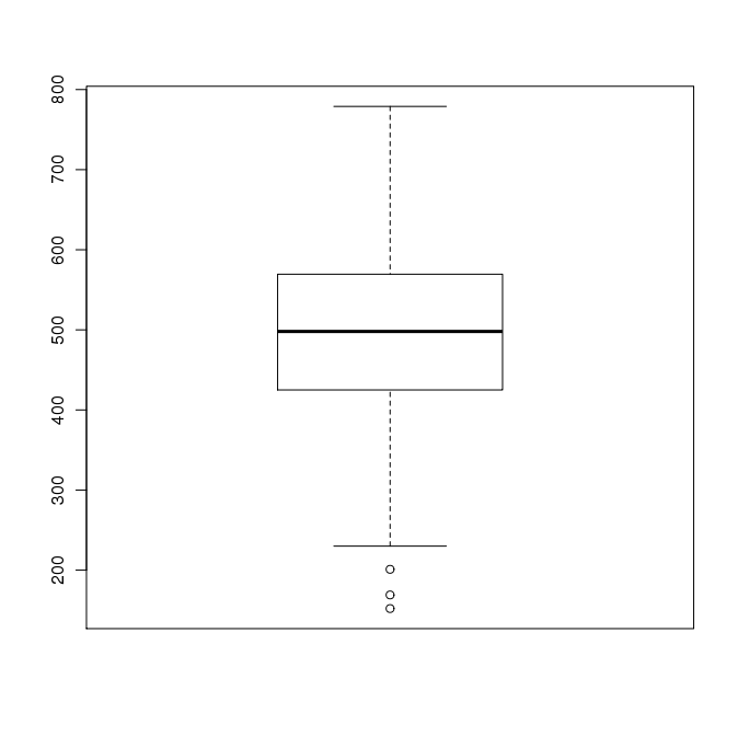
Before we run the analysis, we have to check for outliers. There are two R routines that can be useful. The first is called a boxplot, and it produces a graphical summary called a box-and-whisker plot of the data. This consists of a rectangular box with "whiskers" that extend some distance above and below the box, and finally dots representing outliers.

Enter: boxplot(x) This should produce a graph something like this:

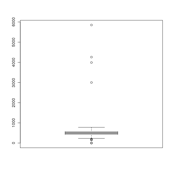
Interpretation is somewhat subjective, but generally if the box and whiskers occupy only a small part of the graph and there are circles representing data points well beyond the whiskers, it indicates the presence of outliers in the data.

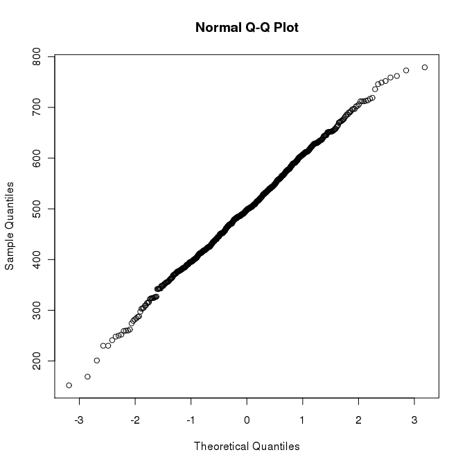
Another useful tool for spotting outliers is the q-q plot.

Enter: qqnorm(x) This should produce a graph something like this:

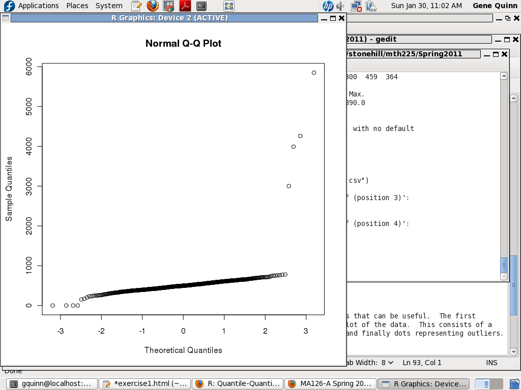
Again the interpretation is subjective, but circles way out of line with the dark part of the graph usually indicate outliers.

In this case, we can be sure any values below 100 and above 800 are invalid, and if the graphs indicate that such values exist in the data, we should remove them.

In general, this is a tedious manual process with careful consideration given to each value discarded. Ideally, we should be able to explain the error, as in the examples of the clams filled with sand. Perhaps zeroes were entered for missing scores, or an extra digit was typed by mistake.

Begin by listing the array of scores with the command x, and visually search for questionable values.

If you decide that an element should be discarded, make sure you have the correct index first by displaying the data value. For example, if we think x[254] is invalid, type

x[254]

to display that data element alone. If it is indeed invalid, replace it by NA using the statement

x[254]<-NA

Be careful not do discard any good values accidentally by typing the wrong index.

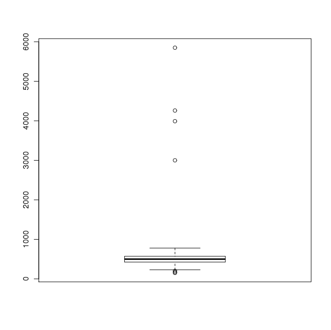
If you have removed all values less than 100, the boxplot should look something like

and the q-q plot something like

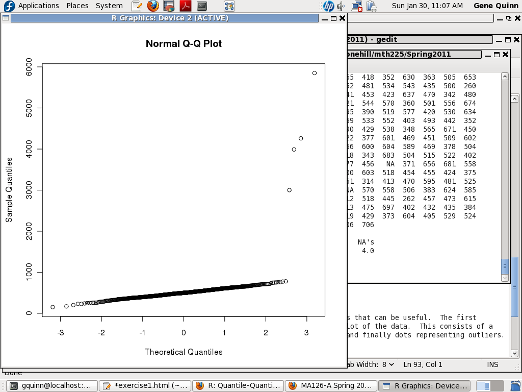
Both of these still indicate outliers, and from the scale we can see there are values greater than 800. So we have to find and remove these. When we have removed all values less than 100 or greater than 800, the plots should look something like

Note that the box and whiskers fill most of the chart, and there are only a few circles outside the whiskers. Also the scale indicates there are no values below 100 or above 800.

Note that the circles are now in a much more linear configuration, and there are now values below 100 or above 800.

At this point, we have completed the data cleanup and are ready to compute the descriptive statistics. The rest of the procedure is identical to Exercise0.

To compute the mean, median, min, max, and first and third quartiles, we can use the summary() function:

summary(x)

(be sure to use the name of the vector and not the name of the data frame here). To compute the standard deviation, last time we used

sd(x)

If we enter this, because there are missing values, the result will be NA. To tell R we want to remove or ignore the missing values, the syntax is:

sd(x,na.rm=TRUE)

Finally, in similar fashion the interquartile range is obtained using

IQR(x,na.rm=TRUE)

Use these values to answer the questions posted on eLearn as Exercise 1.